Abstract
This project:
- Designed a simple model that includes both heat transfer and convection phenomena, where the shape, size parameters, and physical boundary conditions can be altered within a certain range
- Conducted a sweep study using the Design Manager feature of Star-CCM+.
- Utilized Java programming and the sweep functionality of Design Manager to compute 183,750 cases.
- Saved the input and output data of this model into a single dataset.
- Allowed for experiments in future machine learning.
- Ultimately, through machine learning on the dataset, developed a neural network model capable of predicting the thermal performance of the model under various parameters.
- Verified that with sufficient data, valuable outcomes can be achieved by combining machine learning with engineering applications.
Hardware and Software Resources
Software:
- Star-CCM+
- 3D-CAD
- Automation
- Design Manager
- Java
- Jupyter Notebook
- pandas
- numpy
- matplotlib
- pytorch
Hardware:
- PC
- CPU with 6 or more cores
- 8G RAM
- GPU
Simulation Model
The model is shown in the following figure:
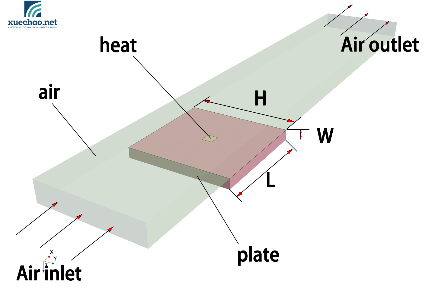
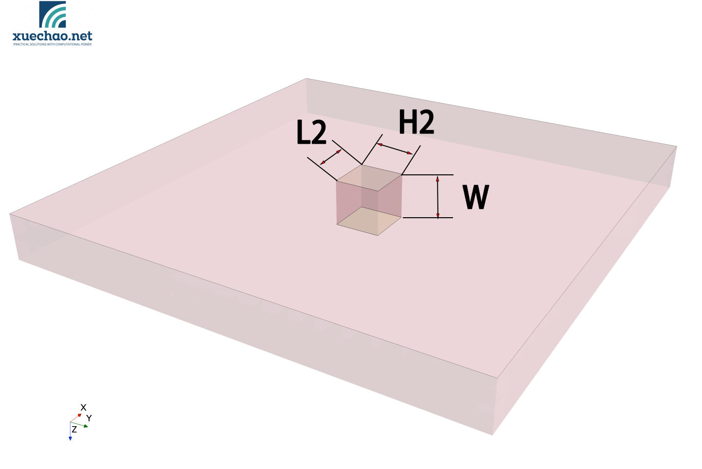
The model is composed of threee parts:
- heat
- plate
- air
heat: The part of heat source, with material properties set to copper, is tightly connected to the plate with no thermal resistance between them. Its length, width, and height are defined as variable dimensions.
plate:Non-heating, with material properties set to iron, its length and width are variable dimensions, while its height remains consistant with the heat source part.
air:Fluid region, with inlet velocity as a variable , but temperature is constant.
This simple model is that the heat part generate a certain amount of heat, with the majority being transfer to the plate through contact, and then dissipated into the air by convection. A small portion of the heat is directly transfered to the air by convection at the top surface of the heat part.
This heat transfer model includes the following 7 variables:
- H ——The width of the plate,range [50,150]mm
- L ——The length of the plate, range [50,150]mm
- W ——The thickness of the plate,range [5,20]mm
- H2 ——The width of the heat,range [5,20]mm
- L2 ——The length of the heat,range [5,20]mm
- v_air ——The inlet velocity of the air,range [5,20]m/s
- heat ——The amount of the heat generation of the heat part,range [1,20]w
Dataset
The dataset can be downloaded from this address.
The explaination of the variable names in the dataset is as follows:
- Design# :The design number of each Star-CCM+ design case.
- “Name” :The name of each Star-CCM+ design case.
- “T_d” :The temperature difference between the air inlet and outlet.
- “T_inlet (C)” :The temperature of the air inlet.
- “T_outlet (C)” :The temperature of the air outlet.
- “energy_out” :The heat carried away by the air through convection, calculated based on the temperature difference between the air inlet and outlet.
- “heatT (C)” :The average temperature of the heat part.
- “mass (kg/s)” :The mass flow rate of the air.
- “Performance” :The performance evaluation of a single design by DM is not meaningful, as we only collect data using the sweep funciton.
- “H (mm)” :The width of the plate.
- “H2 (mm)” :The width of the heat part.
- “L (mm)” :The length of the plate.
- “L2 (mm)” :The length of the heat part.
- “W (mm)” :The thickness of the plate.
- “Wair (mm)” :The thickness of the air setting as a constant.
- “heat” :The amount of the heat generation of the heat part.
- “v”:The inlet velocity of the air.
Machine Learning
Import the dataset into the Notebook and do some cleaning, and select inputs and output.
df.columns
Index(['Design#', 'Name', 'T_d', 'T_inlet(C)', 'T_outlet(C)', 'energy_out',
       'heatT(C)', 'mass(kg/s)', 'Performance', 'H(mm)', 'H2(mm)', 'L(mm)',
       'L2(mm)', 'W(mm)', 'Wair(mm)', 'heat', 'v'],
      dtype='object')
selected_columns = [ 'H(mm)', 'H2(mm)', 'L(mm)','L2(mm)', 'W(mm)',  'heat', 'v','heatT(C)']
df =df[selected_columns]
df.head()
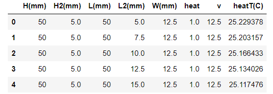
df.describe()

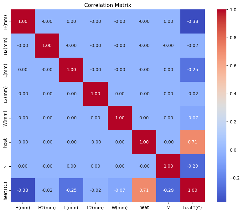
The linear correlation among the dataset variables is shown in the following figure.
Perform linear regression using scikit-learn(SK-learn):
model=LinearRegression()
model.fit(X_train,y_train)
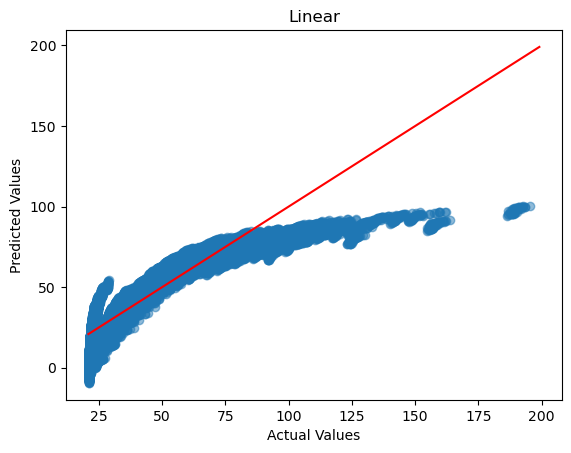
In the test set, the correspondence between predicted values and actual values is as follows:
The evaluation of prediciton accuracy on the test set is as follows:
R2 score:  0.7899667696453285
Mean Squared Error:  104.53257228500799
Mean Absolute Error:  6.8060228938554435
Training with a neural network:
The neural network model primarily employs linear connections and ReLU activation functions.
- The neural network structure consists of 1 input layer, 7 hidden layers, and 1 output layer.
- Using multiple hidden layers with sufficient neurons in each layer allows us to model complex physical phenomena.
- By using the ReLU activation function, we can simulate non-linear phenomena in heat transfer and convection.
def create_model_more_hidden_layers(num_input_cols,num_output_cols):
    model=nn.Sequential(
    nn.Linear(num_input_cols,10),
    nn.ReLU(),
    nn.Linear(10,50),
    nn.ReLU(),
    nn.Linear(50,100),
    nn.ReLU(),
    nn.Linear(100,100),
    nn.ReLU(),
    nn.Linear(100,100),
    nn.ReLU(),
    nn.Linear(100,100),
    nn.ReLU(),
    nn.Linear(100,50),
    nn.ReLU(),
    nn.Linear(50,10),
    nn.ReLU(),
    nn.Linear(10,num_output_cols) # Output Layer with 1 neuron
    )
    return model
num_input_cols = X_train.shape[1]
num_output_cols=1
num_epochs=10000
learning_rate=0.0001
model= create_model_more_hidden_layers(num_input_cols,num_output_cols).to(device)
train_test_model(model,X_train,y_train,X_test,y_test,num_epochs,learning_rate)
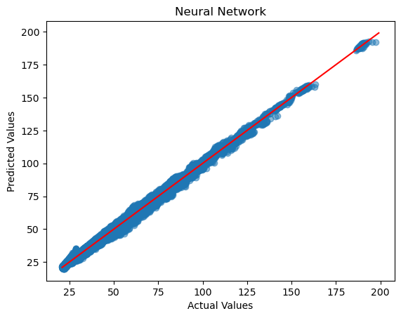
In the test set, the correspondence between predicted values and actual values is as follows:
The evaluation of prediciton accuracy on the test set is as follows:
R2 score:  0.9957430057650765
Mean Squared Error:  2.1337025
Mean Absolute Error:  1.0782065
Conclusion
Through the entire research process of a simple heat transfer and convection model described above, it is evident that using neural networks for machine learning can train effective models for predicting complex physical phenomena.
While the data used in this project was obtained through extensive calculations, conducting machine learning with simulation-generated data holds significant importance for several reasons:
-
Richness of Data: Simulation can generate large volumes of diverse data, crucial for training complex machine learning models, especially when lack of real-world data or it’s costly to obtain.
-
Cost-effectiveness: Generating simulation data is often less costly compared to collecting data in the real world, and it can be generated in large quantities within a short period.
-
Control: Simulations allow precise control over vairiables, facilitating the study of specific conditions’ impact on model performance, which aids in model optimization and validation.
-
Coverage of Extreme Cases: Simulations can simulate extreme scenarios that are rare in real-world situations, provideing comprehensive training data for machine learning models to enhance performance across varous conditions.
Further Considerations
-
It has been verified that using a large amount of data reflecting model features for machine learning can form a complete closed loop. We can leverage any accumulated engineering data to re-understand and reinterpret it through machine learning, and even train machine models for new optimized design calculations.
-
This simple model is indeed very basic, with a very small overall mesh size. Calculating approximately 180,000 sets of data took about 2-3 weeks. If a more complex model has a slightly larger mesh size and each case takes more than ten minutes to compute, then isn’t it impossible to obtain such a large dataset?
