CFD and Machine Learning Part 2: A Slightly More Complex Model - Chapter 2. A Single Variable(SK-Learn)

Abstract

In the previous article, the model used in this study was introduced. In this chapter:

• To explore from the most fundamental and simplified perspective, one of the eight variable parameters of the model was selected for study.
• Different value ranges were defined to study the variable’s behavior across various ranges.
• Sweep calculations were performed to obtain the dataset.
• The analysis of the dataset is based on a physical understanding of the phenomena described by the model.
• Machine learning techniques were then applied, using different models for fitting.
• The goal was to evaluate the performance of different regression models on the dataset.

Model

The model has been introduced in the previous article, as shown in the figure below:

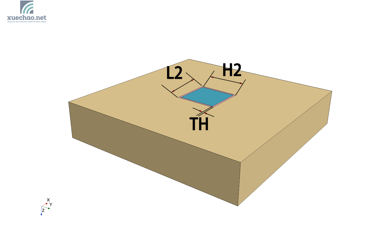
This heat transfer model has 8 adjustable parameters:

• H —— width of the plate,
• L —— length of the plate,
• W —— thickness of the plate,
• H2 —— width of the heat component,
• L2 —— length of the heat component,
• TH —— thickness of the resist layer,
• v_air —— inlet velocity of the air,
• heat —— heat generation rate of the heat component.

Study of A Single Variable

In this chapter, we select only one parameter as the variable, while the other parameters remain constant. The cross-section of the model is shown in the figure below:

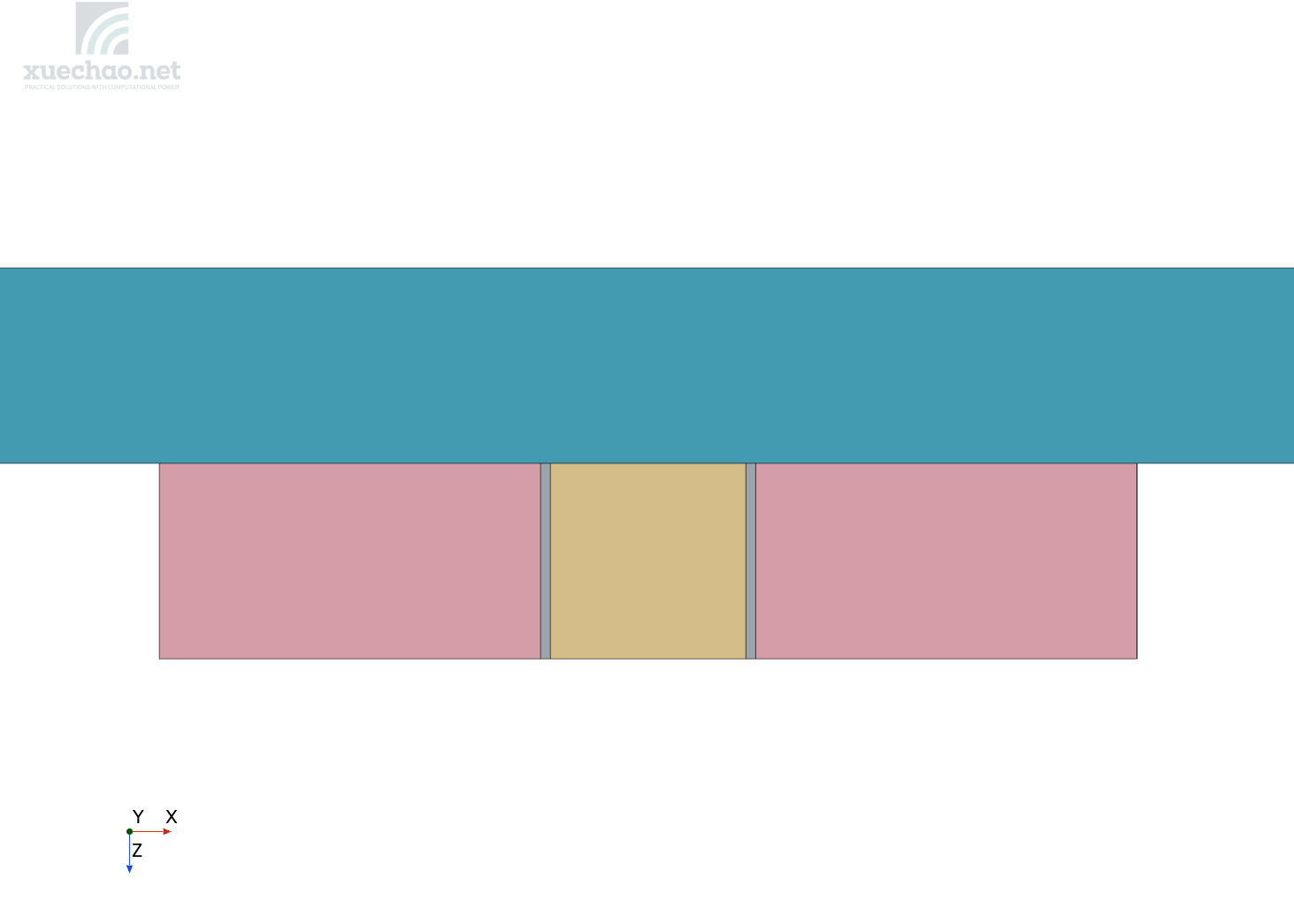
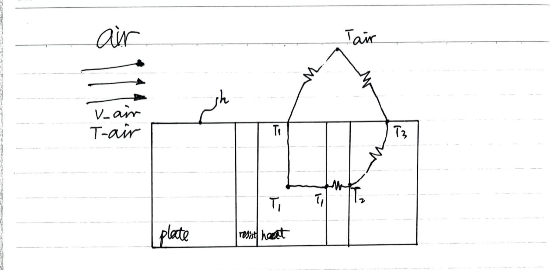
The physical phenomenon reflected by the model has been introduced in our previous article: “A certain amount of heat is emitted from the ‘heat’ component. Most of this heat first passes through the ‘resist,’ which has a relatively low thermal conductivity, and is then transferred to the ‘plate.’ From there, it is dissipated into the air through convective heat transfer between the ‘plate’ and the ‘air.’ A smaller portion of the heat from the ‘heat’ component is directly dissipated into the ‘air’ through convective heat transfer from the top surface of the ‘heat’.”

If we ignore the convective exchange between the ‘resist’ component and the air, as well as some aspects of three-dimensional heat transfer, and assume that the temperature of the ‘heat’ component is uniformly distributed (due to its very high thermal conductivity), we can use a thermal circuit diagram to represent the heat transfer process of this model, as shown in the figure below:

v_air as the variable

First, we will conduct a study with the air velocity v_air as the variable. Based on the thermal circuit diagram above, changes in v_air primarily affect the convective heat transfer coefficient between the air and the solid. According to Newton’s law of cooling: Q = h * A * (Ts - Tf) , the surface temperature of the object is inversely proportional to the convective heat transfer coefficient 1/h.

Using software to calculate the model’s behavior at different air velocities, the relationship between the temperature of the ‘heat’ component and the air velocity is as follows:

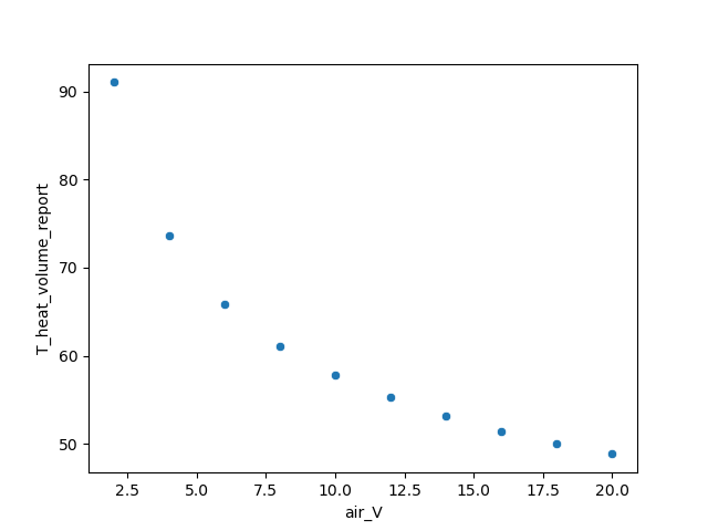
The figure above shows the variation in the average temperature of the ‘heat’ component over the range of air velocities range [2.5, 20] m/s. In this relationship, we can clearly see that the initial analysis using Newton’s law of cooling is consistent with the simulation results. As the air velocity increases, the convective heat transfer coefficient between the air and the solid also increases, which in turn decreases its reciprocal. This results in a nonlinear inverse relationship between air velocity and the temperature of the ‘heat’ component.

If the air velocity ranges from [8, 12] m/s, the temperature variation of the heat component is shown in the figure below:

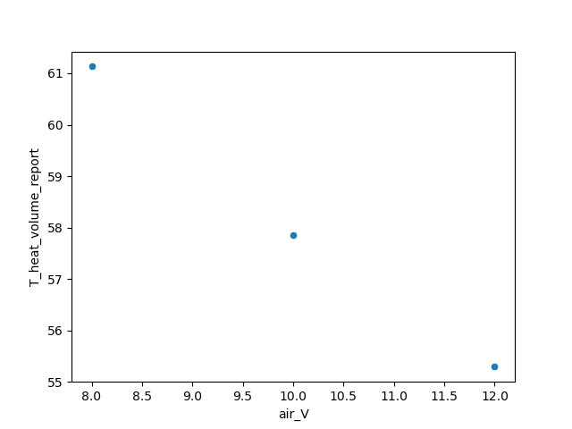
From the above, it can be observed that the strength of the linear relationship between a variable and the result variable varies within different ranges of that variable.

The transverse position of the heat component as a variable

Above, we examined the relationship between the heat temperature and the velocity of the cooling air, which exhibited an inverse proportionality. To generate more complex data, we introduced an additional variable, D, in the original model to describe the transverse position of the heat component, as indicated by the red circle in the figure below:

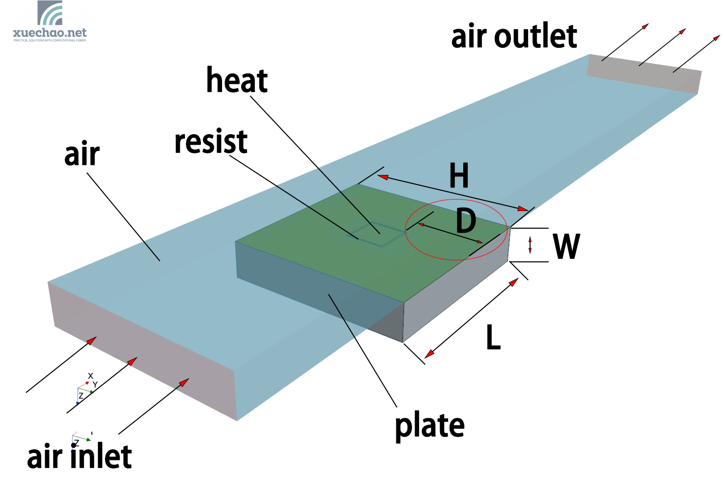
The heat component has a positional variation in the direction perpendicular to the cooling air flow, with its distance from the side edge of the plate being D. The figure below shows a schematic of the model for three different values of D:

We kept D as the sole variable in the model while keeping other parameters constant, and calculated multiple cases with different values of D, ultimately forming the corresponding dataset.

The relationship between the temperature of the heat component and D is shown in the figure below:

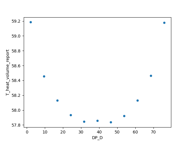
In this model, with only the parameter D as the variable, the primary factor affecting the temperature of the heat component is the size of D, which reflects the relative position of the heat component. If the heat component is positioned closer to the edge, as shown in the cross-sectional temperature distribution in the figure below, one side of the heat component is nearer to the edge. The heat exchange on this side is influenced by the temperature gradient of the plate, leading to a reduced thermal conductivity on that side and consequently increasing the temperature of the heat component.

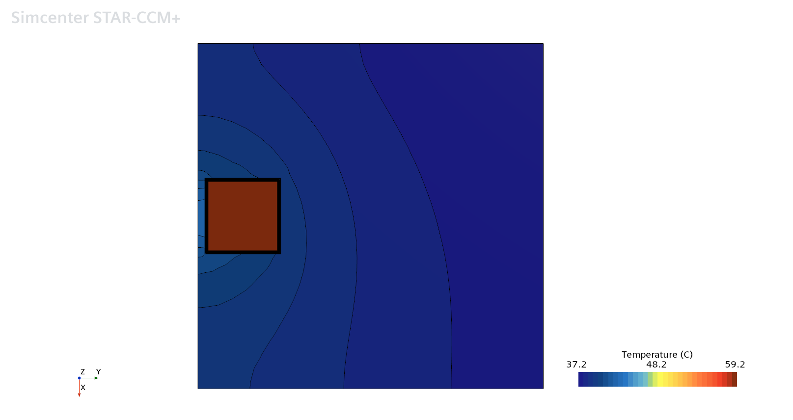
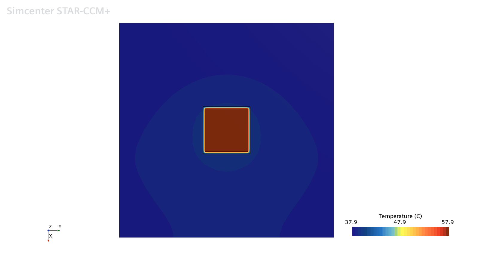
As D gradually increases, the heat component moves towards the center, improving its side heat transfer capability. Therefore, when the heat component is positioned in the center, its temperature is the lowest. The figure below shows the temperature distribution of the heat component when it is located in the central position.

Machine learning study of the dataset with the transverse position of the heat component as a variable

Scikit-learn Linear Regression

First, we use Scikit-learn’s linear fitting method to fit the dataset. It is important to emphasize that we already know that there is no linear relationship between parameter D and the temperature T of the heat component. However, we will give it a try anyway.

model=LinearRegression()
model.fit(X_train,y_train)

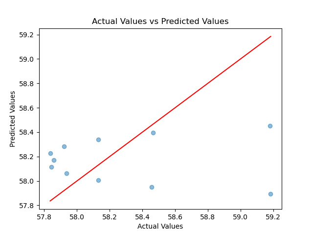
We use the dataset obtained by scanning and computing with CFD software, using this parameter as a variable, as the research object. We train the model using Scikit-learn’s linear regression, and the accuracy of the predictions made by the trained model is shown in the following figure:

The distribution of D vs. T for the actual results and predicted results is shown in the following figure:

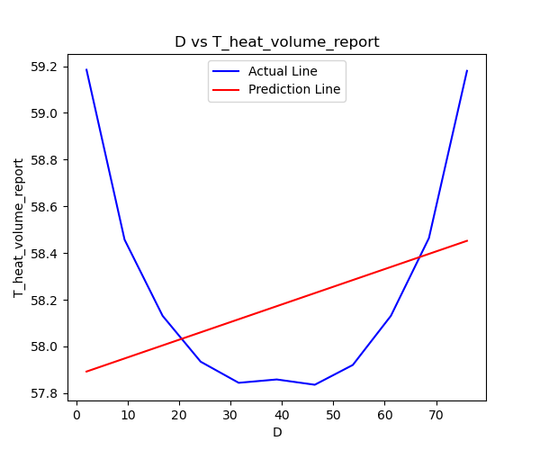
We can clearly see that, from the perspective of physical phenomena, the relationship between D and T is nonlinear. Therefore, linear fitting cannot be used to train the data.

Scikit-learn Polynomial Regression

Since we already know from physical phenomena that the relationship between D and T is not linear, and from the above results, we can see that D and T approximately have a parabolic relationship, we can use Scikit-learn’s polynomial regression to train the dataset.

First, we use a 2nd-degree polynomial, as we have just guessed that the relationship between D and T is likely to be parabolic.

model = make_pipeline(PolynomialFeatures(degree=2), LinearRegression())
model.fit(X_train,y_train)

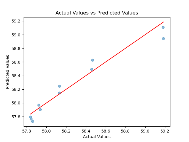
The accuracy of the trained model’s predictions is shown in the following figure:

The distribution of D vs. T for the actual results and predicted results is shown in the following figure:

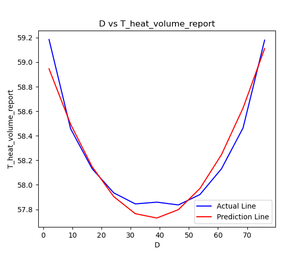
Wow, using a 2nd-degree polynomial regression performs much better than linear regression. However, there is still some error. So let’s try increasing the degree of the polynomial.

The accuracy of the predictions made by the 3rd-degree polynomial regression model is shown in the following figure:

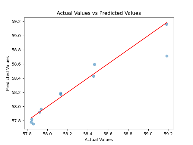
The distribution of D vs. T for the actual results and predicted results with the 3rd-degree polynomial regression is shown in the following figure:

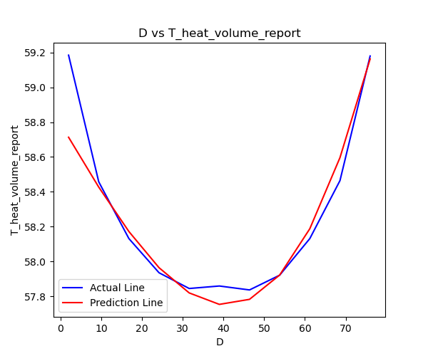
Using the 3rd-degree polynomial regression yields better results than the 2nd-degree polynomial regression.

The accuracy of the predictions made by the 4th-degree polynomial regression model is shown in the following figure:

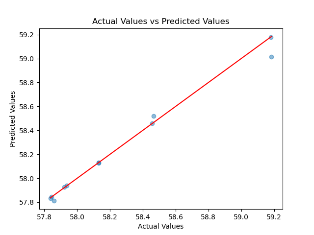The distribution of D vs. T for the actual results and predicted results with the 3rd-degree polynomial regression is shown in the following figure:

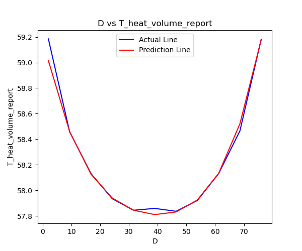
From the above figure, it can be seen that the 4th-degree polynomial regression has performed very well.

Conclusion

This chapter explored two approaches for studying a parameter as a variable in a slightly more complex heat transfer and convection model:

• Physical Phenomena Approach: Starting from the theory of heat transfer and convection, the relationship between the variable and the results was investigated based on physical phenomena.

• Machine Learning Approach: Using data-driven methods, both simple linear regression and polynomial regression were applied to study the dataset.

Understanding the physical phenomena thoroughly can greatly assist in selecting appropriate machine learning models and improving their accuracy.

In the next chapter (Chapter 3), we will use neural networks to study the dataset and compare the results with polynomial regression.