Abstract In the previous article, the accuracy of the model in this study using SK-Learn was introduced. In this chapter:
-
The dataset from the previous chapter was fitted using neural networks,
-
The results were compared with those obtained using SK-Learn,
-
The performance of the neural network model on this dataset was evaluated.
Model
The model has already been introduced in the previous article.
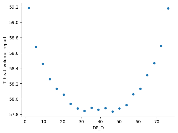
In the earlier article, only one parameter was selected as a variable, while other parameters were kept constant. In this study, an additional variable, D, was introduced to the original model to describe the position of the heat component. To better suit the requirements of neural network models for datasets, we used a dataset containing 21 computed results.
The relationship between the temperature of the heat component and D is shown in the figure below:
Neural Network Study
In the previous article, “CFD and Machine Learning (1): A Simple Model,” we used a neural network structure consisting of one input layer, seven hidden layers, and one output layer. This neural network effectively fitted a model to handle the physical phenomena of our simple model.
So, how should the structure of a neural network be determined? How many layers are considered appropriate? How should the number of neurons in each layer be determined? In the engineering field, for example, how should the structure of a neural network be chosen for a slightly more complex heat transfer model like ours?
We will explore these questions in the following chapters, aiming to gain some insights into using neural networks with engineering data.
SK-Learn Polynomial Regression
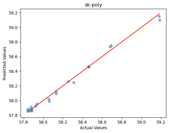
In the previous chapter, we used a 4th-degree polynomial regression to train the model, and the prediction results were very good. The accuracy is shown in the figure below:
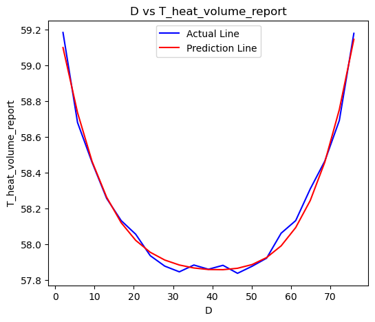
The distribution of the true results versus the predicted results for D vs. T is shown in the figure below:
Neural Networks
We then used a neural network for fitting. The neural network model primarily utilized linear connections and ReLU activation functions. By introducing activation functions, we aimed to simulate nonlinear phenomena.
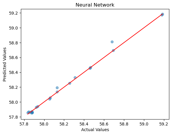
We trained and predicted the same dataset using the previously mentioned neural network, which has seven hidden layers. The accuracy is shown in the figure below:
The distribution of the true results versus the predicted results for D vs. T is shown in the figure below:
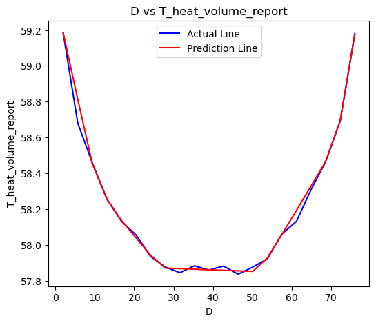
We can see that the neural network also performs very well on this dataset.
Conclusion
In this chapter, we examined a slightly more complex heat transfer and convection model with one parameter as a variable. We used neural networks to study the dataset and compared the results with polynomial regression. It is evident that the regression accuracy of the neural network is also very high. A sufficiently complex neural network can simulate complex physical phenomena effectively.
In the next chapter, we will compare polynomial regression and neural networks in terms of their requirements for dataset size.
